Running Experiments in Parallel with Tune

Try it out

Run this example in the Anyscale Console or view it on GitHub.

⏱️ Time to complete: 10 min

Ray Tune lets you easily run experiments in parallel across a cluster.

In this tutorial, you will learn:

1. How to set up a Ray Tune app to run an parallel grid sweep across a cluster.
2. Basic Ray Tune features, including stats reporting and storing results.
3. Monitoring cluster parallelism and execution using the Ray dashboard.

Note: This tutorial is run within a workspace. Please overview the Introduction to Workspaces template first before this tutorial.

Grid search hello world

Let's start by running a quick "hello world" that runs a few variations of a function call across a cluster. It should take about 10 seconds to run:

from ray import tune

def f(config):
    print("hello world from variant", config["x"])
    return {"my_result_metric": config["x"] ** 2}

tuner = tune.Tuner(f, param_space={"x": tune.grid_search([0, 1, 2, 3, 4])})
results = tuner.fit()
print(results)

Interpreting the results

You should see during the run a table of the trials created by Tune. One trial is created for each individual value of x in the grid sweep. The table shows where the trial was run in the cluster, how long the trial took, and reported metrics:

On completion, it returns a ResultGrid object that captures the experiment results. This includes the reported trial metrics, the path where trial results are saved:

ResultGrid<[
  Result(
    metrics={'my_result_metric': 0},
    path='/home/ray/ray_results/f_2024-02-27_11-40-53/f_1e2c4_00000_0_x=0_2024-02-27_11-40-56',
    filesystem='local',
    checkpoint=None
  ),
  ...

Note that the filesystem of the result says "local", which means results are written to the workspace local disk. We'll cover how to configure Tune storage for a distributed run later in this tutorial.

Viewing trial outputs

To view the stdout and stderr of the trial, use the Logs tab in the Workspace UI. Navigate to the log page and search for "hello", and you'll be able to see the logs printed for each trial run in the cluster:

Tune also saves a number of input and output metadata files for each trial to storage, you can view them by querying the returned result object:

• params.json: The input parameters of the trial
  • params.pkl pickle form of the parameters (for non-JSON objects)
• result.json: Log of intermediate and final reported metrics
  • progress.csv: CSV form of the results
  • events.out.tfevents: TensorBoard form of the results

import os

# Print the list of metadata files from trial 0 of the previous run.
os.listdir(results[0].path)

CIFAR parameter sweep

Next, we'll configure Tune for a larger-scale run on a multi-node cluster. We'll customize the following parameters:

• Resources to request for each trial
• Saving results to cloud storage

We'll also update the function to do something more interesting: train a computer vision model. The following cell defines the training function for CIFAR (adapted from this more complete example).

Note that validation results are reported for each epoch:

from cifar_utils import load_data, Net

import torch
import torch.nn as nn
import torch.nn.functional as F
import torch.optim as optim
from torch.utils.data import random_split

def train_cifar(config):
    net = Net(config["l1"], config["l2"])

    device = "cpu"
    if torch.cuda.is_available():
        device = "cuda:0"
        if torch.cuda.device_count() > 1:
            net = nn.DataParallel(net)
    net.to(device)

    criterion = nn.CrossEntropyLoss()
    optimizer = optim.SGD(net.parameters(), lr=config["lr"], momentum=0.9)

    trainset, _ = load_data("/mnt/local_storage/cifar_data")

    test_abs = int(len(trainset) * 0.8)
    train_subset, val_subset = random_split(
        trainset, [test_abs, len(trainset) - test_abs])

    trainloader = torch.utils.data.DataLoader(
        train_subset,
        batch_size=int(config["batch_size"]),
        shuffle=True,
        num_workers=0,
    )
    valloader = torch.utils.data.DataLoader(
        val_subset,
        batch_size=int(config["batch_size"]),
        shuffle=True,
        num_workers=0,
    )

    for epoch in range(5):  # loop over the dataset multiple times
        running_loss = 0.0
        epoch_steps = 0
        for i, data in enumerate(trainloader):
            # get the inputs; data is a list of [inputs, labels]
            inputs, labels = data
            inputs, labels = inputs.to(device), labels.to(device)

            # zero the parameter gradients
            optimizer.zero_grad()

            # forward + backward + optimize
            outputs = net(inputs)
            loss = criterion(outputs, labels)
            loss.backward()
            optimizer.step()

            # print statistics
            running_loss += loss.item()
            epoch_steps += 1
            if i % 2000 == 1999:  # print every 2000 mini-batches
                print("[%d, %5d] loss: %.3f" % (epoch + 1, i + 1,
                                                running_loss / epoch_steps))
                running_loss = 0.0

        # Validation loss
        val_loss = 0.0
        val_steps = 0
        total = 0
        correct = 0
        for i, data in enumerate(valloader, 0):
            with torch.no_grad():
                inputs, labels = data
                inputs, labels = inputs.to(device), labels.to(device)

                outputs = net(inputs)
                _, predicted = torch.max(outputs.data, 1)
                total += labels.size(0)
                correct += (predicted == labels).sum().item()

                loss = criterion(outputs, labels)
                val_loss += loss.cpu().numpy()
                val_steps += 1

        train.report(
            {"loss": (val_loss / val_steps), "accuracy": correct / total},
        )
    print("Finished Training")

The code below walks through how to parallelize the above training function in Tune. Go ahead and run the cell, it will take 5-10 minutes to complete on a multi-node cluster. While you're waiting, go ahead and proceed to the next section to learn how to monitor the execution.

It will sweep across several choices for "l1", "l2", and "lr" of the net:

from filesystem_utils import get_path_and_fs
from ray import tune, train
import os

# Define where results are stored. We'll use the Anyscale artifact storage path to
# save results to cloud storage.
STORAGE_PATH = os.environ["ANYSCALE_ARTIFACT_STORAGE"] + "/tune_results"
storage_path, fs = get_path_and_fs(STORAGE_PATH)

# Define trial sweep parameters across l1, l2, and lr.
trial_space = {
    "l1": tune.grid_search([8, 16, 64]),
    "l2": tune.grid_search([8, 16, 64]),
    "lr": tune.grid_search([5e-4, 1e-3]),
    "batch_size": 4,
}

# Can customize resources per trial, including CPUs and GPUs.
# You can try changing this to {"gpu": 1} to run on GPU.
train_cifar = tune.with_resources(train_cifar, {"cpu": 2})

# Start a Tune run and print the output.
tuner = tune.Tuner(
    train_cifar,
    param_space=trial_space,
    run_config=train.RunConfig(storage_path=storage_path, storage_filesystem=fs),
)
results = tuner.fit()
print(results)

During and after the execution, Tune reports a table of current trial status and reported accuracy. You can find the configuration that achieves the highest accuracy on the validation set:

Persisted result storage

Because we set storage_path to $ANYSCALE_ARTIFACT_STORAGE/tune_results, Tune will upload trial results and artifacts to the specified storage.

We didn't save any checkpoints in the example above, but if you setup checkpointing, the checkpoints would also be saved in this location:

# Note: On GCP cloud use `gsutil ls` instead.
!aws s3 ls $ANYSCALE_ARTIFACT_STORAGE/tune_results/

Monitoring Tune execution in the cluster

Let's observe how the above run executed in the Ray cluster for the workspace. To do this, go to the "Ray Dashboard" tab in the workspace UI.

First, let's view the run in the Jobs sub-tab and click through to into the job view. Here, you can see an overview of the job, and the status of the individual actors Tune has launched to parallelize the job:

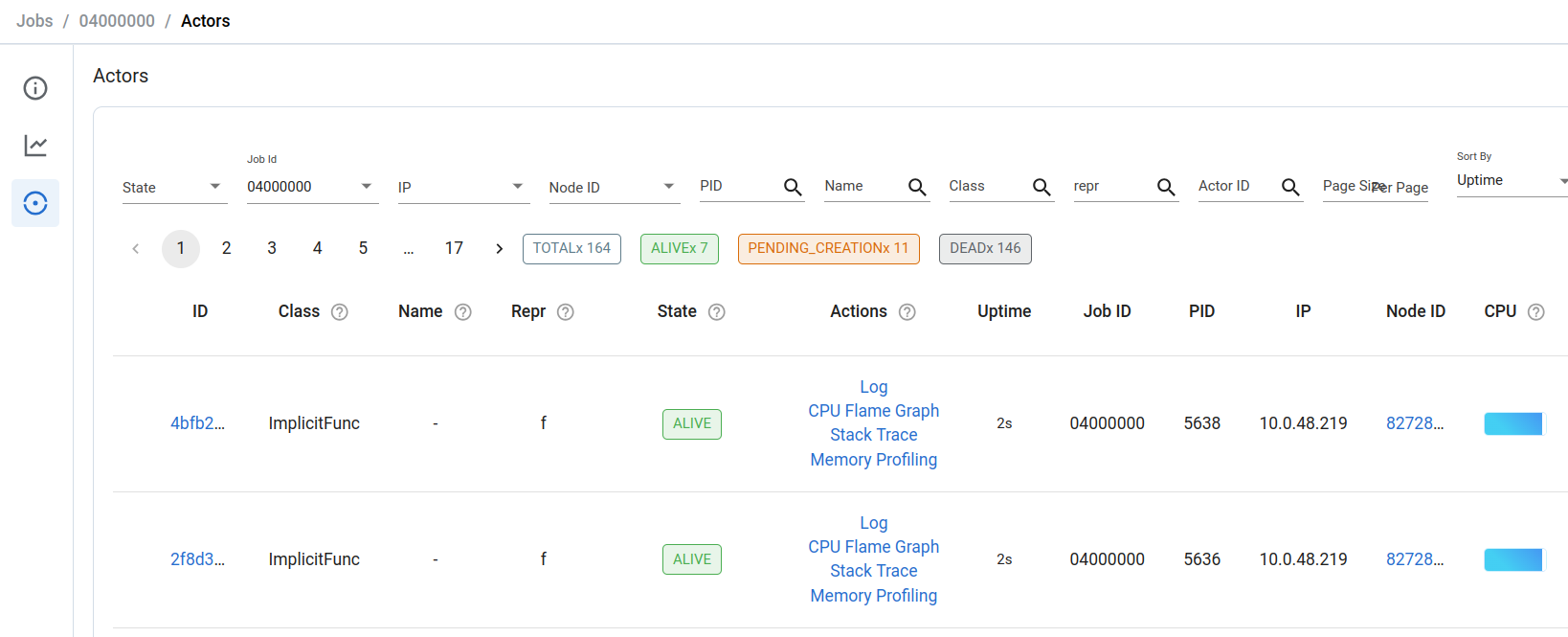
You can further click through to the actors sub-page and view the status of individual running actors. Inspect trial logs, CPU profiles, and memory profiles using this page:

Finally, we can observe the holistic execution of the job in the cluster in the Metrics sub-tab. When running the above job on a 36-CPU cluster, we can see that Tune was able to launch ~16 concurrent actors for trial execution, with each actor assigned 2 CPU slots as configured:

That concludes our overview of Ray Tune in Anyscale. To learn more about Ray Tune and how it can improve your experiment management lifecycle, check out the Ray Tune docs.

Summary

This notebook:

• Ran basic parallel experiment grid sweeps in a workspace.
• Showed how to configure Ray Tune's storage and scheduling options.
• Demoed how to use observability tools on a CIFAR experiment run in the cluster.